P3D2: Visualizing space and time
These slides map to the R example slides on Day 25 or P3D11
At 3:45 we have a Zoom meeting with a SafeGraph employee.
In his iconic flow map of Napoleon’s catastrophic 1812 invasion of Russia, Charles Joseph Minard blends and bends temporal and spatial representations. The path and number of outward-bound soldiers is represented by an initially thick tan ribbon while the dwindling numbers of retreating survivors are represented by a narrowing black band. In this visualization, the time it took to march into Russia is not clear. The only time stamps shown are for the return trip and progressing from right to left. In a sense, time is “bent” to advance the impact of the visual narrative.

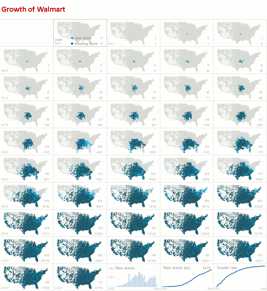
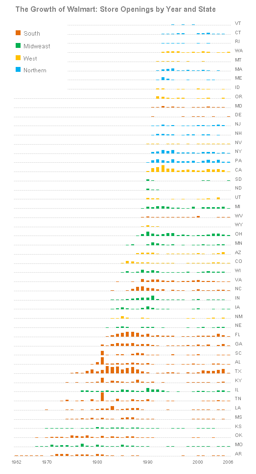
Small multiples (facets) and time
Animated
Questions and data
Spatial mapping
Amelia McNamara and spatial polygons
- 2:37 Gelman on maps and variables
- 11:07 Modifiable areal unit problem
- 12:11 Histogram example
- 14:20 Washinton Post on Gerrymandering
- 14:20 John Oliver on Gerrymandering has some crude language after 6 minutes.
- 16:45 The redistricting game
- 17:40 Talismanic Redistricting
- 19:27 Dasymetric Maps
- 21:10 Mapping upscaling interactive example
- 22:08 Side Scaling: Nested Polygons and redrawing the states
- 23:20 Misaligned Polygons and Flint. Zipcodes are problematic.
- 26:19 Tobler’s First Law
- 27:08 Pycno Package
Handling SafeGraph Data
- Chipotle stores data provided free from ‘When do people visit Chipotle stores? Get your Free Patterns Dataset now thru Oct 10th.’ provided by shop.safegraph.com
- Google Drive Data
- Ohio Restaurants POI
SafeGraphR
library(tidyverse)
library(sf)
library(jsonlite)

json_to_tibble <- function(x){
    if(is.na(x))  return(x)
    parse_json(x) %>%
    enframe() %>%
    unnest(value)
}

bracket_to_tibble <- function(x){
    value <- str_replace_all(x, "\\[|\\]", "") %>%
        str_split(",", simplify = TRUE) %>%
        as.numeric()

    name <- seq_len(length(value))

    tibble::tibble(name = name, value = value)
}
Changing json dictionaries to nested tibbles
dat <- read_csv("SafeGraph - Patterns and Core Data - Chipotle - July 2021/Core Places and Patterns Data/chipotle_core_poi_and_patterns.csv")

datNest <- dat %>%
    slice(1:50) %>% # for the example in class.
    mutate(
        open_hours = map(open_hours, ~json_to_tibble(.x)),
        visits_by_day = map(visits_by_day, ~bracket_to_tibble(.x)),
        visitor_country_of_origin = map(visitor_country_of_origin, ~json_to_tibble(.x)),
        bucketed_dwell_times = map(bucketed_dwell_times, ~json_to_tibble(.x)),
        related_same_day_brand = map(related_same_day_brand, ~json_to_tibble(.x)),
        related_same_month_brand = map(related_same_month_brand, ~json_to_tibble(.x)),
        popularity_by_hour = map(popularity_by_hour, ~json_to_tibble(.x)),
        popularity_by_day = map(popularity_by_day, ~json_to_tibble(.x)),
        device_type = map(device_type, ~json_to_tibble(.x)),
        visitor_home_cbgs = map(visitor_home_cbgs, ~json_to_tibble(.x)),
        visitor_home_aggregation = map(visitor_home_aggregation, ~json_to_tibble(.x)),
        visitor_daytime_cbgs = map(visitor_daytime_cbgs, ~json_to_tibble(.x))
        )
datNest <- datNest %>%
    select(placekey, latitude, longitude, street_address,
        city, region, postal_code,
        raw_visit_counts:visitor_daytime_cbgs, parent_placekey, open_hours)
Python
# %%
import pandas as pd
import numpy as np
# %%
raw_url = 'https://raw.githubusercontent.com/ryanfoxsquire/demodata/master/ohioRestaurants/Starter-OH-Restaurants-CORE_POI-2019-08-09/Starter-OH-Restaurants-CORE_POI-2019-08-09.csv'
dat = pd.read_csv(raw_url)